
Visualizing Tropical Storm Colin Precipitation using geoknife
Using the R package geoknife to plot precipitation by county during Tropical Storm Colin.
Tropical Storm Colin (TS Colin) made landfall on June 6 in western
Florida. The storm moved up the east coast, hitting Georgia, South
Carolina, and North Carolina. We can explore the impacts of TS Colin
using open data and R. Using the USGS-R geoknife package, we can pull
precipitation data by county.
First, we created two functions. One to fetch data and one to map data.
Function to retrieve precip data using
geoknife
:
Function to map cumulative precipitation data using R package maps:
Now, we can use those functions to fetch data for specific counties and time periods.
TS Colin made landfall on June 6th and moved into open ocean on June 7th. Use these dates as the start and end times in our function (need to account for timezone, +5 UTC). We can visualize the path of the storm by mapping cumulative precipitation for each county.
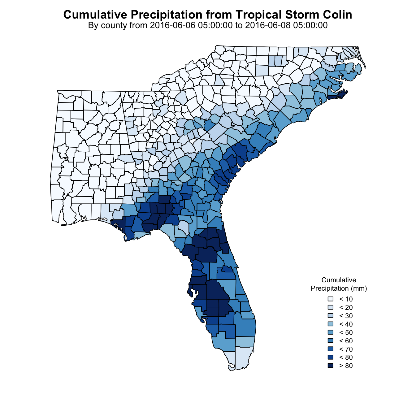
Map of precipitation
Questions
Please direct any questions or comments on geoknife to:
https://github.com/DOI-USGS/geoknife/issues
Edited on 11/23/2018. Works with geoknife v1.4.0 on CRAN. Changes to fips retrieval to use US Census data based on changes for this geoknife issue .
Edited on 11/09/2020 to update data source and county data
Categories:
Related Posts
The Hydro Network-Linked Data Index
November 2, 2020
Introduction updated 11-2-2020 after updates described here . updated 9-20-2024 when the NLDI moved from labs.waterdata.usgs.gov to api.water.usgs.gov/nldi/ The Hydro Network-Linked Data Index (NLDI) is a system that can index data to NHDPlus V2 catchments and offers a search service to discover indexed information.
Accessing LOCA Downscaling Via OPeNDAP and the Geo Data Portal with R.
September 13, 2016
Introduction In this example, we will use the R programming language to access LOCA data via the OPeNDAP web service interface using the ncdf4 package then use the geoknife package to access LOCA data using the Geo Data Portal as a geoprocessing service.
Seasonal Analysis in EGRET
November 29, 2016
Introduction This document describes how to obtain seasonal information from the R package EGRET . For example, we might want to know the fraction of the load that takes place in the winter season (say that is December, January, and February).
Calculating Moving Averages and Historical Flow Quantiles
October 25, 2016
This post will show simple way to calculate moving averages, calculate historical-flow quantiles, and plot that information. The goal is to reproduce the graph at this link: PA Graph .
The case for reproducibility
October 6, 2016
Science is hard. Why make it harder? Scientists and researchers spend a lot of time on data preparation and analysis, and some of these analyses are quite computationally intensive.