
Tol Color Schemes
Qualitative, diverging, and sequential color schemes by Paul Tol.
Introduction
Choosing colors for a graphic is a bit like taking a trip down the rabbit hole, that is, it can take much longer than expected and be both fun and frustrating at the same time. Striking a balance between colors that look good to you and your audience is important. Keep in mind that color blindness affects many individuals throughout the world and it is incumbent on you to choose a color scheme that works in color-blind vision. Luckily there are a number of excellent R packages that address this very issue, such as the colorspace , RColorBrewer , and viridis packages. And because this is R, where diversity is king, why not offer one more function for creating color blind friendly palettes.
Let me introduce the GetTolColors function in the R-package
inlmisc
.
This function generates a vector of colors from qualitative, diverging,
and sequential color schemes by Paul Tol (2018)
.
The original inspiration for developing this function came from
Peter Carl’s blog post
describing color schemes from an older issue of Paul Tol’s Technical Note (issue 2.2, released Dec. 2012).
And the qualitative color schemes described in his blog post found their way into the
ptol_pal function in the R-package ggthemes
.
My intent with this document is to exhibit the latest Tol color schemes (issue 3.0, released May 2018) and show
that they are not only visually pleasing but also well thought out.
To get started, install the inlmisc package from CRAN using the command:
And if you’re so inclined, read through the function documentation.
Like almost every other R function used to create a color palette,
GetTolColors takes as its first argument the number of colors to be in the returned palette (n).
For example, the following command generates a palette of 10 colors using default values for function arguments.
##  [1] "#E8ECFB" "#B997C7" "#824D99" "#4E78C4" "#57A2AC" "#7EB875" "#D0B541"
##  [8] "#E67F33" "#CE2220" "#521A13"
## attr(,"bad")
## [1] "#666666"
## attr(,"call")
## GetTolColors(n = 10, scheme = "smooth rainbow", alpha = NULL,
##     start = 0, end = 1, bias = 1, reverse = FALSE, blind = NULL,
##     gray = FALSE)
## attr(,"class")
## [1] "Tol"       "character"
Returned from the function is an object of class "Tol" that inherits behavior from the "character" class.
A Tol-class object is comprised of a character vector of n colors and the following attributes:
"names", the informal names assigned to colors in the palette,
where a value of NULL indicates that no color names were specified for the scheme;
"bad", the color meant for bad data or data gaps, where a value of NA indicates
that no bad color was specified for the scheme; and
"call", the unevaluated function call that can be used to reproduce the palette.
A plot method is provided for the Tol class that displays the palette of colors.
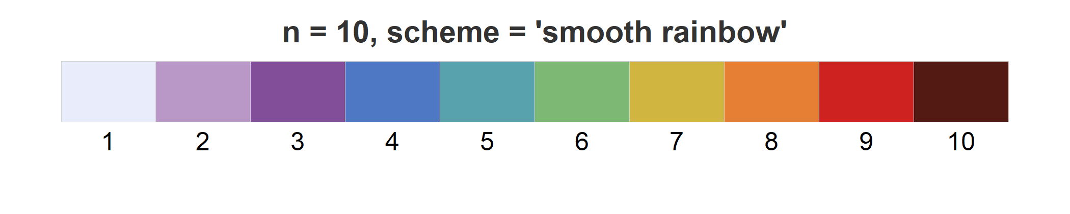
Display colors in palette.
The main title for the plot will always indicate the n and scheme argument values used to create the palette.
Where scheme is the name of the color scheme, its default value is "smooth rainbow".
All other arguments are only included in the title if their specified value differs from their default value.
The label positioned below each shaded rectangle gives the informal color name.
Color Schemes
Tal (2018) defines 13 color schemes:
7 for qualitative data, 3 for diverging data, and 3 for sequential data (table 1).
The maximum number of colors in a generated palette is dependent on the user selected scheme.
For example, the "discrete rainbow" scheme can have at most 23 colors in its palette (n ≤ 23).
Whereas a continuous (or interpolated) version of the "smooth rainbow" scheme is available that has
no upper limit on values of n.
About half of the schemes include a color meant for bad data.
| Data type | Color scheme | Maximum n | Bad data |
|---|---|---|---|
| Qualitative | bright | 7 (3) | no |
| vibrant | 7 (4) | no | |
| muted | 9 (5) | yes | |
| pale | 6 | no | |
| dark | 6 | no | |
| light | 9 | no | |
| ground cover | 14 | no | |
| Diverging | sunset | --- | yes |
| BuRd | --- | yes | |
| PRGn | --- | yes | |
| Sequential | YlOrBr | --- | yes |
| discrete rainbow | 23 | yes | |
| smooth rainbow | --- | yes |
Qualitative
Qualitative color schemes "bright", "vibrant", "muted", "pale", "dark", and "light"
are appropriate for representing nominal or categorical data.
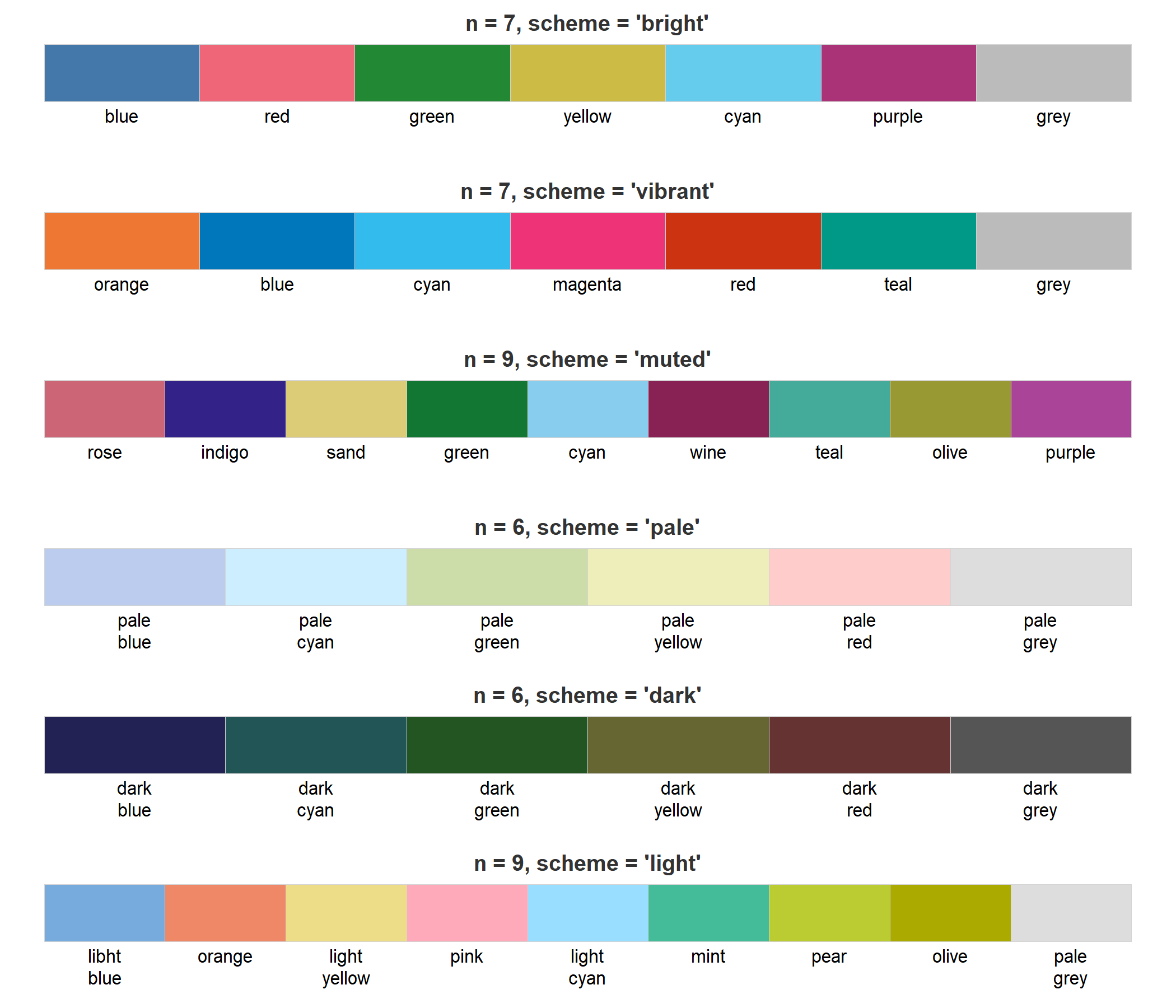
Qualitative color schemes
And the "ground cover" scheme is a color-blind safe version of the
AVHRR
global land cover classification color scheme (Hansen and others, 1998).
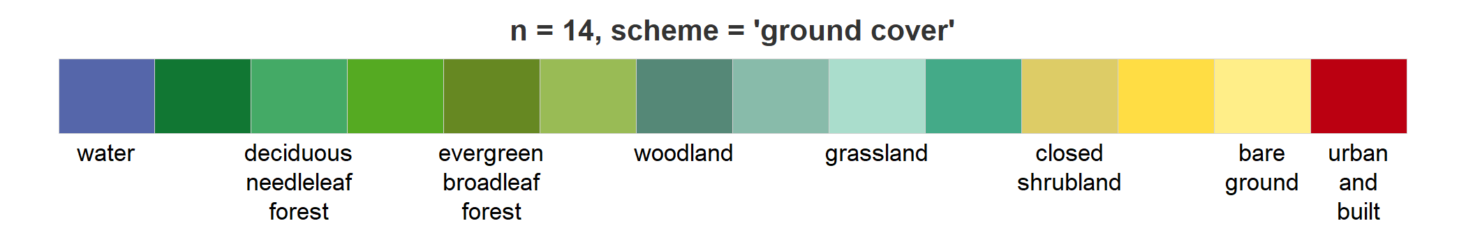
Land cover color scheme
Note that schemes "pale", "dark", and "ground cover" are intended to be accessed
in their entirety and subset using vector element names.
Diverging
Diverging color schemes "sunset", "BuRd", and "PRGn" are appropriate for representing
quantitative data with progressions outward from a critical midpoint of the data range.
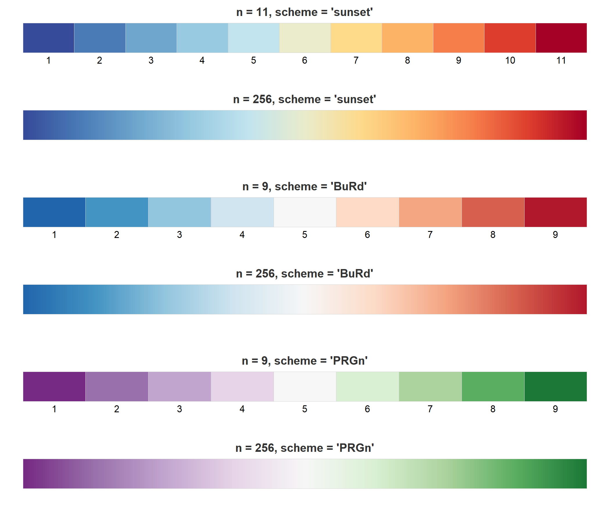
Diverging color schemes
Sequential
Sequential schemes "YlOrBr", "discrete rainbow", and "smooth rainbow" are appropriate for representing
quantitative data that progress from small to large values.

Sequential color schemes
Alpha Transparency
The transparency (or opacity) of palette colors is specified using the alpha argument.
Values range from 0 (fully transparent) to 1 (fully opaque).
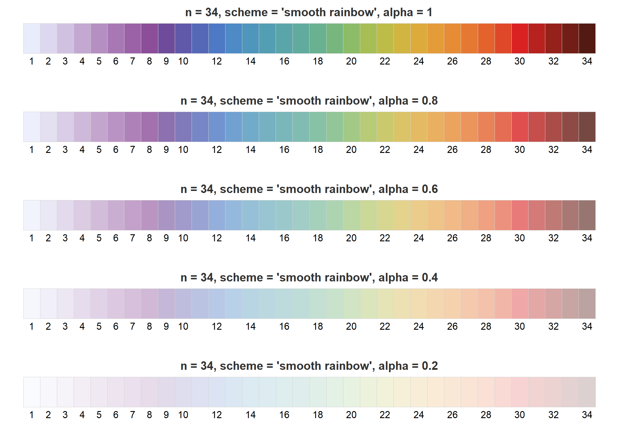
Adjust alpha transparency of colors.
Color Levels
Color levels are used to limit the range of colors in a scheme—applies only to schemes that can be interpolated,
which includes the "sunset", "BuRd", "PRGn", "YlOrBr", and "smooth rainbow" schemes.
Starting and ending color levels are specified using the start and end arguments, respectively.
Values range from 0 to 1 and represent a fraction of the scheme’s color domain.
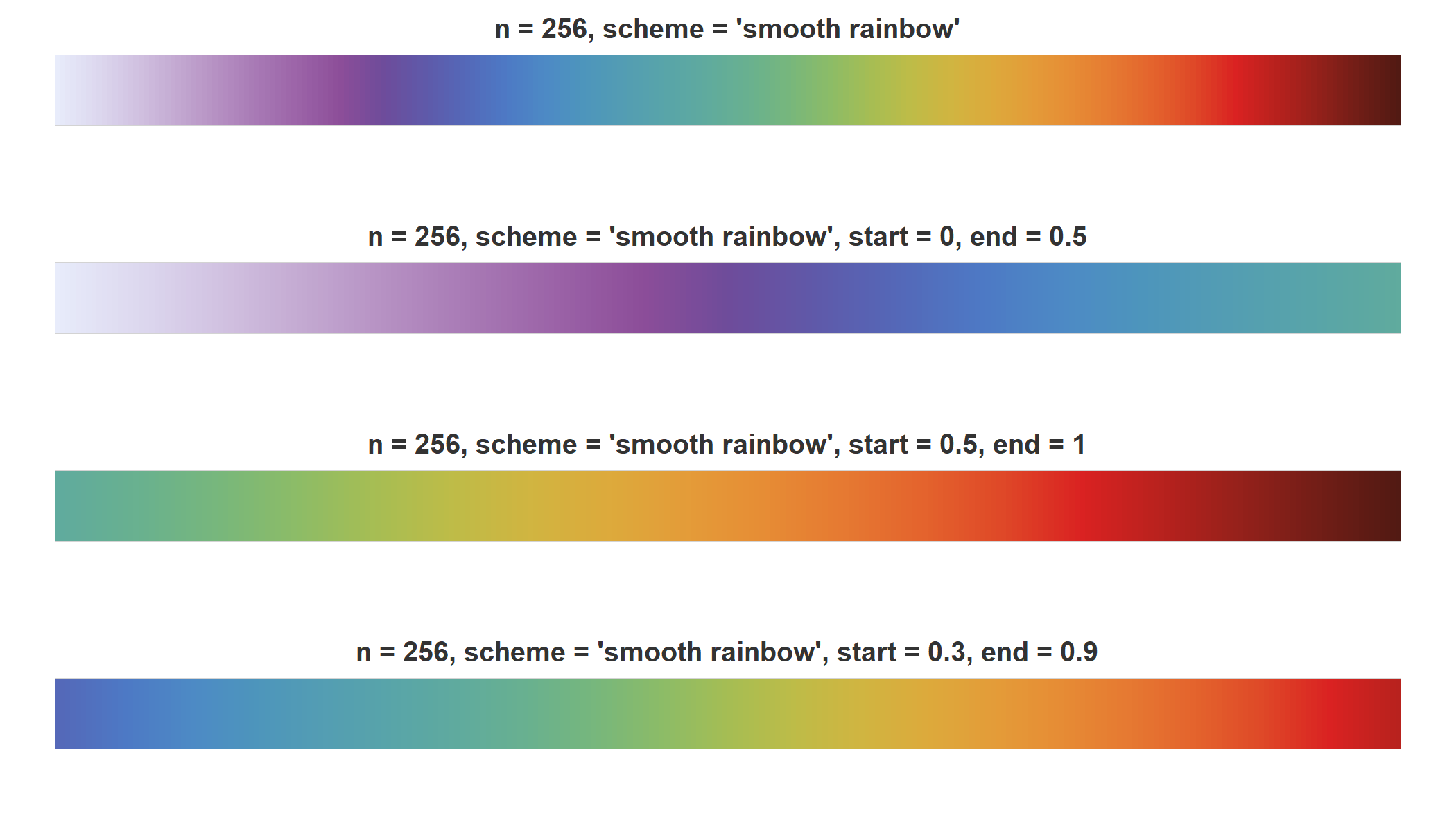
Adjust starting and ending color levels.
Interpolation Bias
Interpolation bias is specified using the bias argument, where a value of 1 indicates no bias.
Smaller values result in more widely spaced colors at the low end,
and larger values result in more widely spaced colors at the high end.
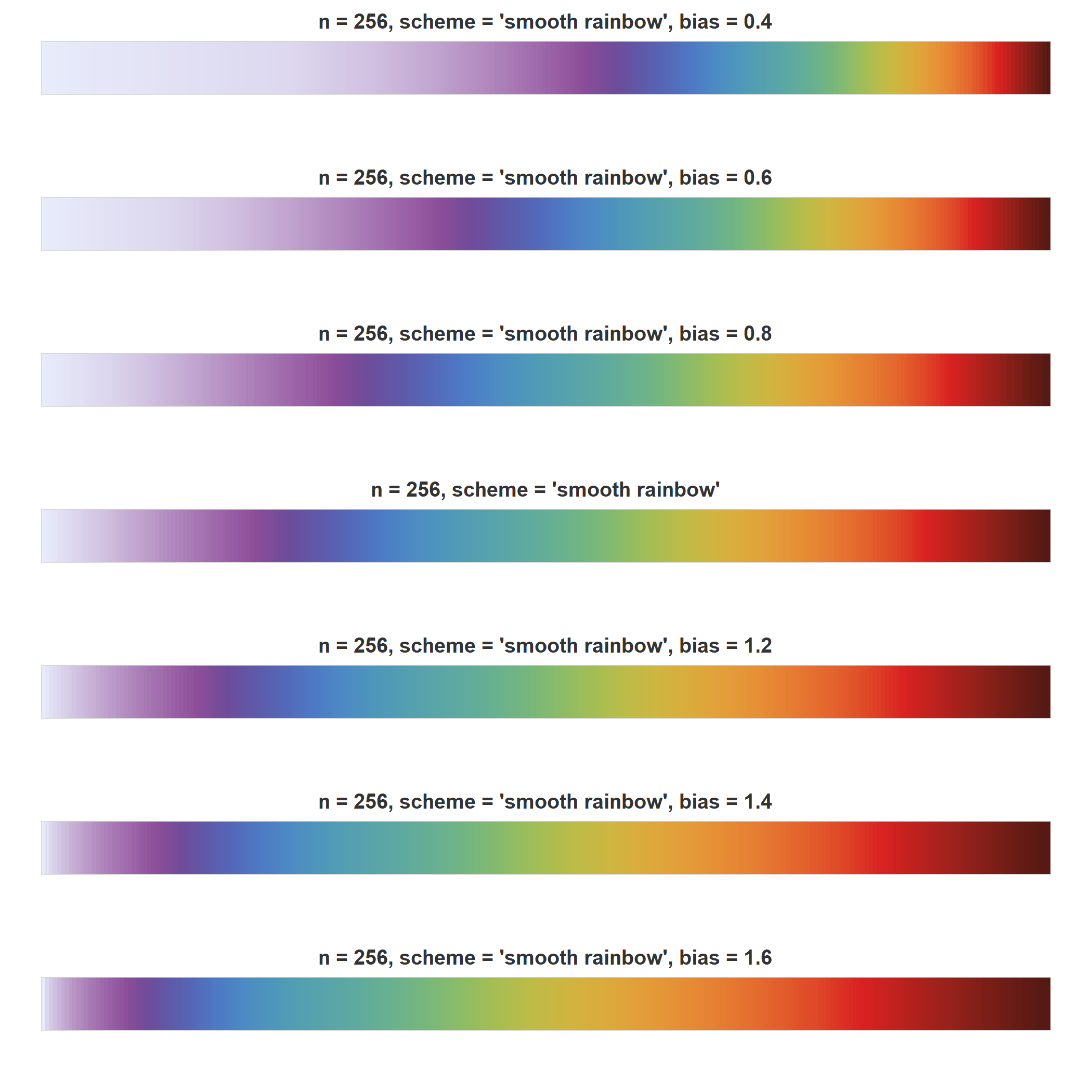
Adjust interpolation bias.
Reverse Colors
Reverse the order of colors in a palette by specifying the reverse argument as TRUE .
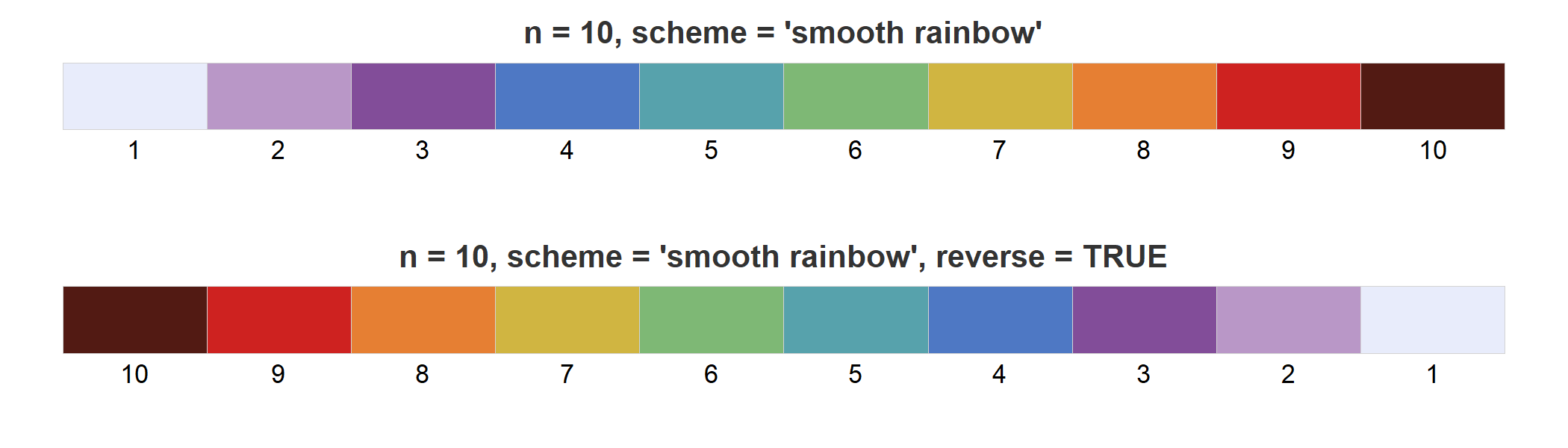
Reverse colors in palette.
Color Blindness
Different types of color blindness can be simulated using the blind argument:
specify "deutan" for green-blind vision, "protan" for red-blind vision,
"tritan" for green-blue-blind vision, and "monochromacy" for total-color blindness.
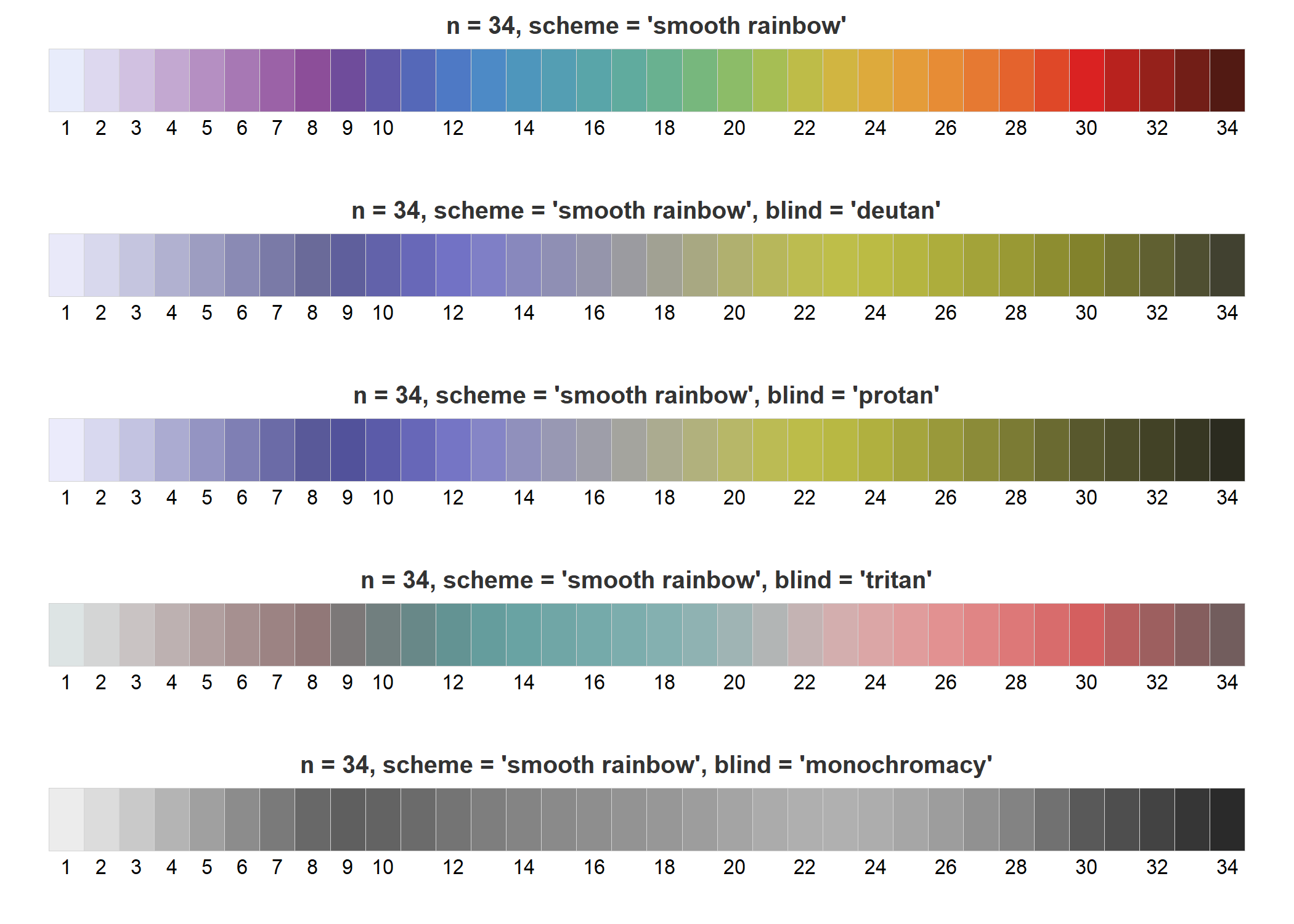
Adjust for color blindness.
With the exception of total-color blindness,
the "smooth rainbow" scheme is well suited for the variants of color-vision deficiency.
Gray-Scale Preparation
Subset the qualitative schemes "bright", "vibrant", and "muted"
to work after conversion to gray scale by specifying the gray argument as TRUE.
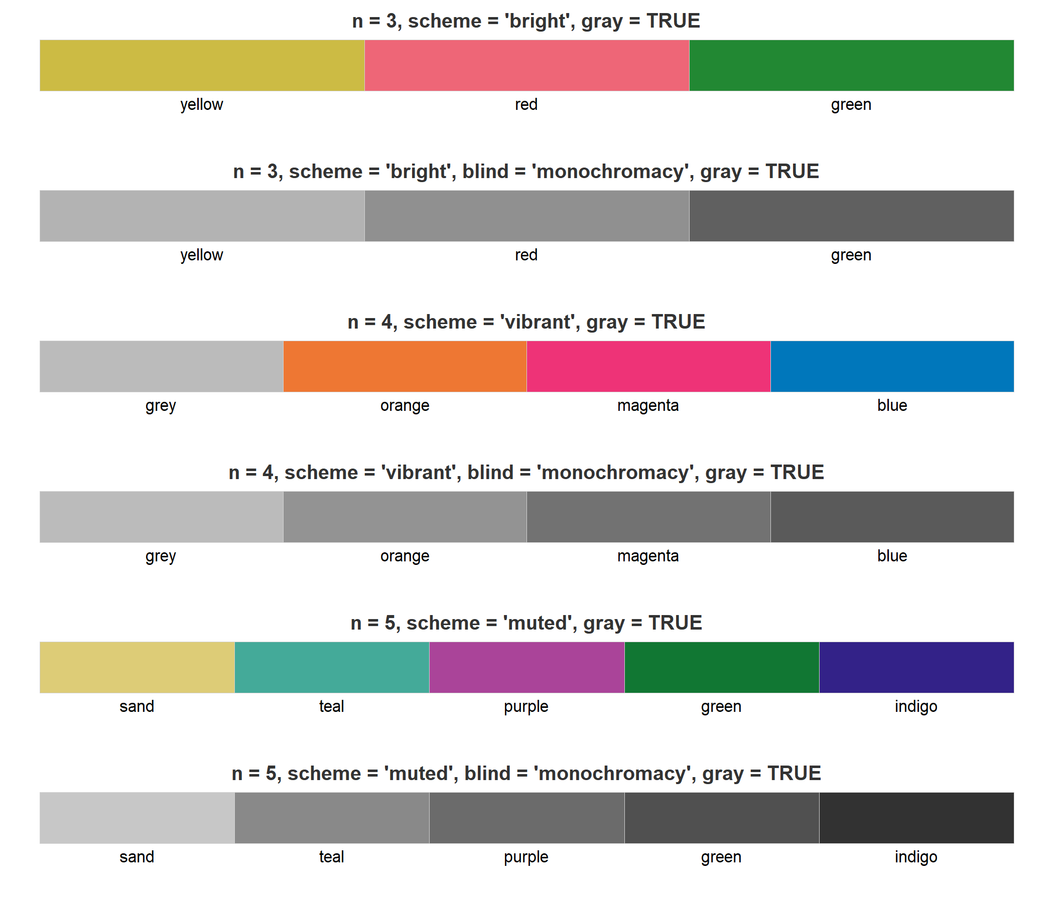
Prepare qualitative schemes for gray-scale conversion.
Note that the sequential scheme "YlOrBr" works well for conversion to gray scale.
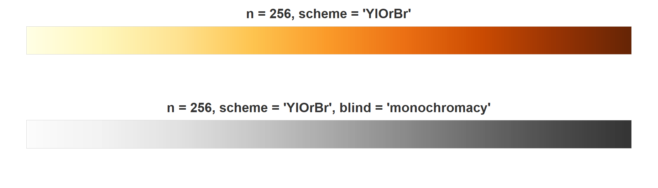
Prepare YlOrBr scheme for gray-scale conversion.
References Cited
Hansen, M., DeFries, R., Townshend, J.R.G., and Sohlberg, R., 1998, UMD Global Land Cover Classification, 1 Kilometer, 1.0: Department of Geography, University of Maryland, College Park, Maryland, 1981-1994.
Tol, Paul, 2018, Colour Schemes: SRON Technical Note, doc. no. SRON/EPS/TN/09-002, issue 3.0, 17 p., accessed August 29, 2018 at https://personal.sron.nl/~pault/data/colourschemes.pdf .
Reproducibility
R-session information for content in this document is as follows:
##  setting  value
##  version  R version 3.5.1 (2018-07-02)
##  system   x86_64, mingw32
##  ui       Rgui
##  language (EN)
##  collate  English_United States.1252
##  tz       America/Los_Angeles
##  date     2018-09-12
##
##  package    * version date       source
##  backports    1.1.2   2017-12-13 CRAN (R 3.5.0)
##  base       * 3.5.1   2018-07-02 local
##  checkmate    1.8.5   2017-10-24 CRAN (R 3.5.1)
##  compiler     3.5.1   2018-07-02 local
##  datasets   * 3.5.1   2018-07-02 local
##  devtools     1.13.6  2018-06-27 CRAN (R 3.5.1)
##  dichromat    2.0-0   2013-01-24 CRAN (R 3.5.0)
##  digest       0.6.16  2018-08-22 CRAN (R 3.5.1)
##  evaluate     0.11    2018-07-17 CRAN (R 3.5.1)
##  graphics   * 3.5.1   2018-07-02 local
##  grDevices  * 3.5.1   2018-07-02 local
##  grid         3.5.1   2018-07-02 local
##  highr        0.7     2018-06-09 CRAN (R 3.5.1)
##  igraph       1.2.2   2018-07-27 CRAN (R 3.5.1)
##  inlmisc      0.4.3   2018-09-10 CRAN (R 3.5.1)
##  knitr        1.20    2018-02-20 CRAN (R 3.5.1)
##  lattice      0.20-35 2017-03-25 CRAN (R 3.5.1)
##  magrittr     1.5     2014-11-22 CRAN (R 3.5.1)
##  memoise      1.1.0   2017-04-21 CRAN (R 3.5.1)
##  methods    * 3.5.1   2018-07-02 local
##  pkgconfig    2.0.2   2018-08-16 CRAN (R 3.5.1)
##  rgdal        1.3-4   2018-08-03 CRAN (R 3.5.1)
##  rstudioapi   0.7     2017-09-07 CRAN (R 3.5.1)
##  sp           1.3-1   2018-06-05 CRAN (R 3.5.1)
##  stats      * 3.5.1   2018-07-02 local
##  stringi      1.2.4   2018-07-20 CRAN (R 3.5.1)
##  stringr      1.3.1   2018-05-10 CRAN (R 3.5.1)
##  tools        3.5.1   2018-07-02 local
##  utils      * 3.5.1   2018-07-02 local
##  withr        2.1.2   2018-03-15 CRAN (R 3.5.1)
Categories:
Related Posts
Maps with inlmisc
July 17, 2018
Introduction This document gives a brief introduction to making static and dynamic maps using inlmisc , an R package developed by researchers at the United States Geological Survey (USGS) Idaho National Laboratory (INL) Project Office .
The Hydro Network-Linked Data Index
November 2, 2020
Introduction updated 11-2-2020 after updates described here . updated 9-20-2024 when the NLDI moved from labs.waterdata.usgs.gov to api.water.usgs.gov/nldi/ The Hydro Network-Linked Data Index (NLDI) is a system that can index data to NHDPlus V2 catchments and offers a search service to discover indexed information.
Furthest Water
September 21, 2018
Finding the Location Furthest from Water in the Conterminous United States The idea for this post came a few months back when I received an email that started, “I am a writer and teacher and am reaching out to you with a question related to a piece I would like to write about the place in the United States that is furthest from a natural body of surface water.
Beyond Basic R - Version Control with Git
August 24, 2018
Depending on how new you are to software development and/or R programming, you may have heard people mention version control, Git, or GitHub. Version control refers to the idea of tracking changes to files through time and various contributors.
Beyond Basic R - Mapping
August 16, 2018
Introduction There are many different R packages for dealing with spatial data. The main distinctions between them involve the types of data they work with — raster or vector — and the sophistication of the analyses they can do.