Beyond Basic R - Mapping
Basic mapping in R with the maps and ggmap package
Introduction
There are many different R packages for dealing with spatial data. The main distinctions between them involve the types of data they work with — raster or vector — and the sophistication of the analyses they can do. Raster data can be thought of as pixels, similar to an image, while vector data consists of points, lines, or polygons. Spatial data manipulation can be quite complex, but creating some basic plots can be done with just a few commands. In this post, we will show simple examples of raster and vector spatial data for plotting a watershed and gage locations, and link to some other more complex examples.
Setting up
First, let’s download an example shapefile (a polygon) of a HUC8 from western Pennsylvania, using the sbtools package to access ScienceBase
. The st_read function from the sf (for “simple features”) package reads in the shapefile. We will be using sf throughout these examples to manipulate the points and polygon for the gages and HUC. Then we’ll retrieve gages with discharge from this watershed using the dataRetrieval package. Both dataRetrieval and sbtools are covered in our USGS Packages curriculum
.
library(sbtools)
library(dataRetrieval)
library(sf)

item_file_download(sb_id = "5a83025ce4b00f54eb32956b",
                   names = "huc8_05010007_example.zip",
                   destinations = "huc8_05010007_example.zip",
                   overwrite_file = TRUE)
## [1] "huc8_05010007_example.zip"
unzip('huc8_05010007_example.zip', overwrite = TRUE)
#note st_read takes the folder, not a particular file
huc_poly <- st_read('huc8_05010007_example')
## Reading layer `wbdhu8_alb_simp' from data source `D:\LADData\RCode\owi-blog\content\huc8_05010007_example' using driver `ESRI Shapefile'
## Simple feature collection with 1 feature and 9 fields
## geometry type:  POLYGON
## dimension:      XY
## bbox:           xmin: -79.45512 ymin: 39.91875 xmax: -78.55573 ymax: 40.77377
## epsg (SRID):    4326
## proj4string:    +proj=longlat +datum=WGS84 +no_defs
class(huc_poly)
## [1] "sf" "data.frame"
str(huc_poly)
## Classes 'sf' and 'data.frame':   1 obs. of  10 variables:
##  $ REGION    : Factor w/ 1 level "Ohio Region": 1
##  $ SUBREGION : Factor w/ 1 level "Allegheny": 1
##  $ BASIN     : Factor w/ 1 level "Allegheny": 1
##  $ SUBBASIN  : Factor w/ 1 level "Conemaugh": 1
##  $ HUC_2     : Factor w/ 1 level "05": 1
##  $ HUC_4     : Factor w/ 1 level "0501": 1
##  $ HUC_6     : Factor w/ 1 level "050100": 1
##  $ HUC_8     : Factor w/ 1 level "05010007": 1
##  $ HU_8_STATE: Factor w/ 1 level "PA": 1
##  $ geometry  :sfc_POLYGON of length 1; first list element: List of 1
##   ..$ : num [1:256, 1:2] -79 -79 -79 -79 -79 ...
##   ..- attr(*, "class")= chr  "XY" "POLYGON" "sfg"
##  - attr(*, "sf_column")= chr "geometry"
##  - attr(*, "agr")= Factor w/ 3 levels "constant","aggregate",..: NA NA NA NA NA NA NA NA NA
##   ..- attr(*, "names")= chr  "REGION" "SUBREGION" "BASIN" "SUBBASIN" ...
st_geometry(huc_poly)
## Geometry set for 1 feature
## geometry type:  POLYGON
## dimension:      XY
## bbox:           xmin: -79.45512 ymin: 39.91875 xmax: -78.55573 ymax: 40.77377
## epsg (SRID):    4326
## proj4string:    +proj=longlat +datum=WGS84 +no_defs
st_bbox(huc_poly)
##      xmin      ymin      xmax      ymax
## -79.45512  39.91875 -78.55573  40.77377
st_crs(huc_poly)
## Coordinate Reference System:
##   EPSG: 4326
##   proj4string: "+proj=longlat +datum=WGS84 +no_defs"
huc_gages <- whatNWISdata(huc = "05010007", parameterCd = "00060", service="uv")
head(huc_gages)
##     agency_cd  site_no                                        station_nm
## 197      USGS 03039925 North Fork Bens Creek at North Fork Reservoir, PA
## 591      USGS 03040000                  Stonycreek River at Ferndale, PA
## 621      USGS 03041029                Conemaugh River at Minersville, PA
## 731      USGS 03041500                     Conemaugh River at Seward, PA
## 824      USGS 03042000                  Blacklick Creek at Josephine, PA
## 964      USGS 03042280                  Yellow Creek near Homer City, PA
##     site_tp_cd dec_lat_va dec_long_va coord_acy_cd dec_coord_datum_cd
## 197         ST   40.26619   -79.01669            S              NAD83
## 591         ST   40.28563   -78.92058            S              NAD83
## 621         ST   40.34139   -78.92611            S              NAD83
## 731         ST   40.41924   -79.02614            S              NAD83
## 824         ST   40.47701   -79.18670            S              NAD83
## 964         ST   40.57257   -79.10337            S              NAD83
##       alt_va alt_acy_va alt_datum_cd   huc_cd data_type_cd parm_cd stat_cd
## 197     <NA>       <NA>         <NA> 05010007           uv   00060    <NA>
## 591  1184.06        .01       NGVD29 05010007           uv   00060    <NA>
## 621     1140        .01       NGVD29 05010007           uv   00060    <NA>
## 731  1076.01        .01       NGVD29 05010007           uv   00060    <NA>
## 824   954.46        .01       NAVD88 05010007           uv   00060    <NA>
## 964     1140        .01       NGVD29 05010007           uv   00060    <NA>
##      ts_id loc_web_ds medium_grp_cd parm_grp_cd  srs_id access_cd
## 197 221326       <NA>           wat        <NA> 1645423         0
## 591 122456       <NA>           wat        <NA> 1645423         0
## 621 122464       <NA>           wat        <NA> 1645423         0
## 731 122468       <NA>           wat        <NA> 1645423         0
## 824 122471       <NA>           wat        <NA> 1645423         0
## 964 122477       <NA>           wat        <NA> 1645423         0
##     begin_date   end_date count_nu
## 197 1987-10-03 1998-09-26     4011
## 591 1991-10-01 2018-08-16     9816
## 621 2001-12-13 2018-08-16     6090
## 731 1991-10-01 2018-08-16     9816
## 824 1991-10-15 2018-08-16     9802
## 964 1991-10-01 2018-08-16     9816
The huc_poly object is a new type of object that we haven’t seen — it has classes sf as well as data.frame. Looking inside the object with the str command, we can see it is structured very much like a data.frame with several factor columns, except for the geometry column, which is of type sfc_POLYGON. sf provides various functions to extract useful information from this kind object, generally prefixed with st_. st_geometry extracts the entire geometry part of the object; st_bbox extracts the bounding box from the geometry; and st_crs extracts the coordinate reference system. There are others, but we will use these three to get the parts of the sf object we need for plotting.
Now that we understand this new object, let’s make some maps.
Raster map example
For the raster map, we will use the ggmap package to create a road and satellite basemaps for the HUC. Since the basemaps that ggmap uses are quite detailed, they are too large to include with the package and must be retrieved from the web with the get_map function. For the location argument, we are getting the bbox from the huc_poly object. st_bbox returns the bbox in the format we need, except for the names, which we add with setNames. The ggmap function is analogous to the ggplot function in the ggplot2 package that you have likely already used. It creates the base map, which we can then add things to. Many of the commands used here are from the ggplot2 package (ggmap imports them), and others could be used to further customize this map.
Note that ggmap is probably not a good choice if you need your data to be in a particular projection. Compared to base plotting, it provides simplicity at the cost of control.
library(ggmap)

bbox <- setNames(st_bbox(huc_poly), c("left", "bottom", "right", "top"))
#setting zoom to 9 gives us a bit of padding around the bounding box
basemap_streets <- get_map(maptype = "roadmap", location = bbox, zoom = 9)
basemap_satellite <- get_map(maptype = "satellite", location = bbox, zoom = 9)
street_map <- ggmap(basemap_streets)
satellite_map <- ggmap(basemap_satellite)
print(street_map)
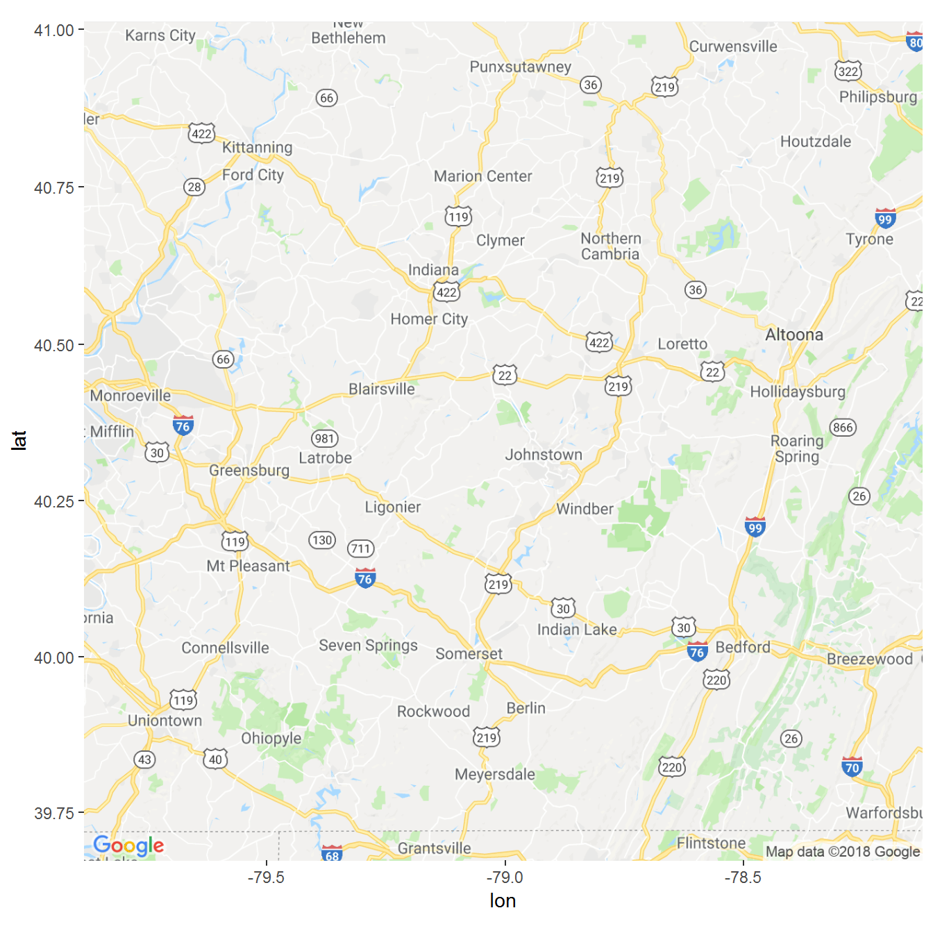
street base map
print(satellite_map)
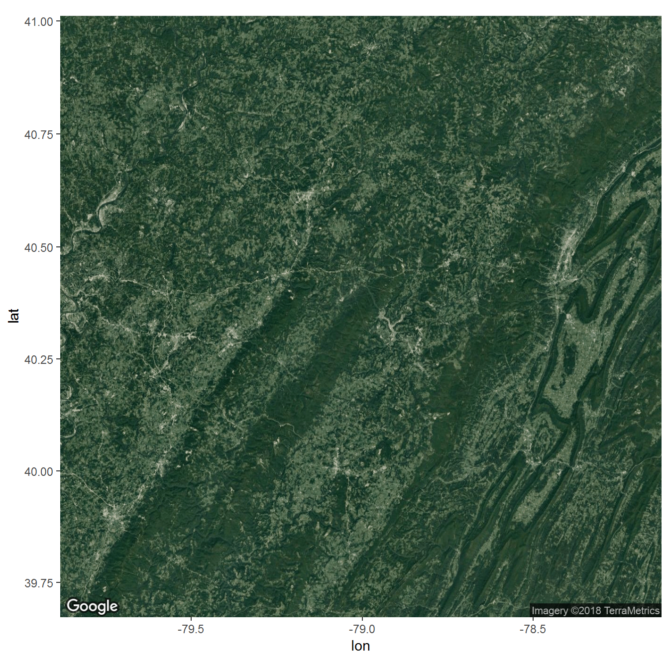
satellite base map
Now we can start adding to our maps. First, we convert the huc_gages data.frame to an sf object using st_as_sf, assigning it the same coordinate reference system as huc_poly using st_crs. ggplot functions like geom_sf and geom_text add to your base map.
huc_gages_sf <- st_as_sf(huc_gages, coords = c("dec_long_va", "dec_lat_va"),
                         crs = st_crs(huc_poly), remove = FALSE)
satellite_map + geom_sf(data = huc_poly,
                        inherit.aes = FALSE,
                        color = "white", fill = NA) +
  geom_sf(data = huc_gages_sf, inherit.aes = FALSE, color = "red") +
  geom_text(data = huc_gages_sf,
            aes(label = site_no, x = dec_long_va, y = dec_lat_va),
            hjust = 0, size=2.5, nudge_x = 0.02, col = "yellow")

satellite map with HUC and gages
street_map + geom_sf(data = huc_poly,
                        inherit.aes = FALSE,
                        color = "black", fill = NA) +
  geom_sf(data = huc_gages_sf, inherit.aes = FALSE, color = "red") +
  geom_text(data = huc_gages_sf, aes(label = site_no, x = dec_long_va, y = dec_lat_va),
             hjust = 0, size=2.5, nudge_x = 0.02, col = "black")
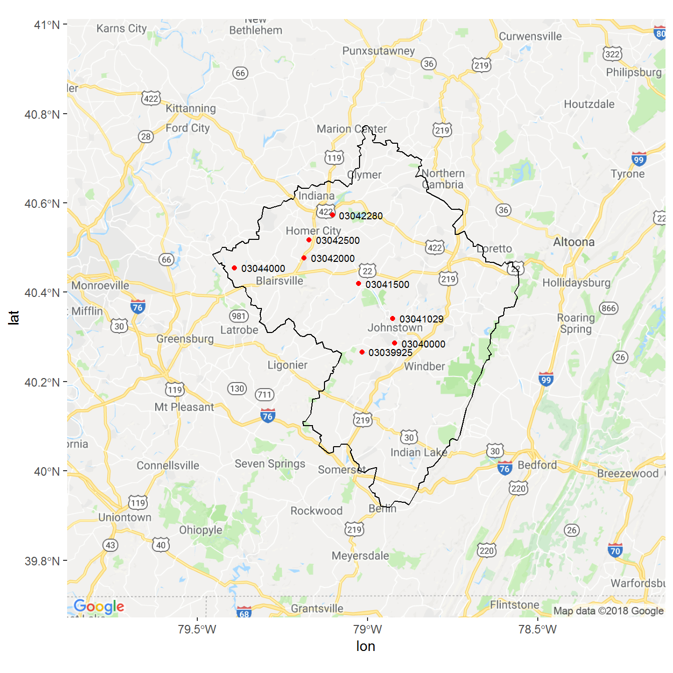
street map with HUC and gages
Vector map example
If we don’t want any raster background to our maps, we can use base plotting and the maps package. This style of map can be nicer for insets or large scale maps that would be cluttered with a raster background. The maps package provides easily accessible political boundary maps, that can be overlaid with other shapefiles. As with regular base plotting, you can think of creating maps like painting — every layer has to go on in the right order. You can’t remove things without starting over. Fortunately, you can start over with just a few keystrokes since you are scripting your plot! Run these commands one by one to see the map take shape — first we create a blank state map, then add county lines in white, then the HUC boundary, then the gage points, and then the legend. Note that we use the st_geometry function inside of the plot command so that we only plot the huc_poly and huc_gages_sf geometry, and not the other information in their data frames.
library(maps)
map(database = 'state', regions = 'Pennsylvania', col = "tan", fill = TRUE, border = NA)
#this draws all PA counties since the regions argument uses partial matching
map(database = 'county', regions = 'Pennsylvania', col = "white", fill = FALSE, add = TRUE)
plot(st_geometry(huc_poly), col = NA, add = TRUE)
plot(st_geometry(huc_gages_sf), add = TRUE, col = "red", pch = 19, cex = 0.7)
legend("bottomright", legend = c("Gage", "Subbasin boundary"), pch = c(19,NA), lty = c(NA, 1),
       col = c("red", "black"), title = "Legend")
title("Conemaugh Subbasin")
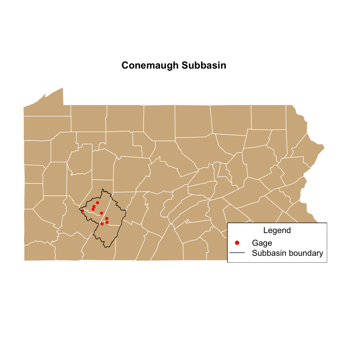
Polygon map of Pennsylvania
Similarly, we can create a map zoomed in to the HUC polygon. Note that we set the x and y limits of the map by extracting the limits of the bbox object we created earlier. We can use the names left, right, etc. because bbox is a named vector.
  map(database = 'county', regions = 'Pennsylvania', col = "lightgray",
      xlim = bbox[c('left', 'right')], ylim = bbox[c('bottom', 'top')])
 plot(st_geometry(huc_poly), col = "dodgerblue", border = NA, add = TRUE)
  box()
 plot(st_geometry(huc_gages_sf), add = TRUE, col = "red", pch = 19, cex = 0.7)
  legend("bottomleft", legend = c("Gage", "Conemaugh subbasin"), pch = c(19,NA), lty = c(NA, 1),
       col = c("red", "dodgerblue"), title = "Legend", lwd = c(1,15), bg = "wheat")
  text(x = huc_gages$dec_long_va, y = huc_gages$dec_lat_va, labels = huc_gages$site_no,
       pos = 4, cex = 0.7)
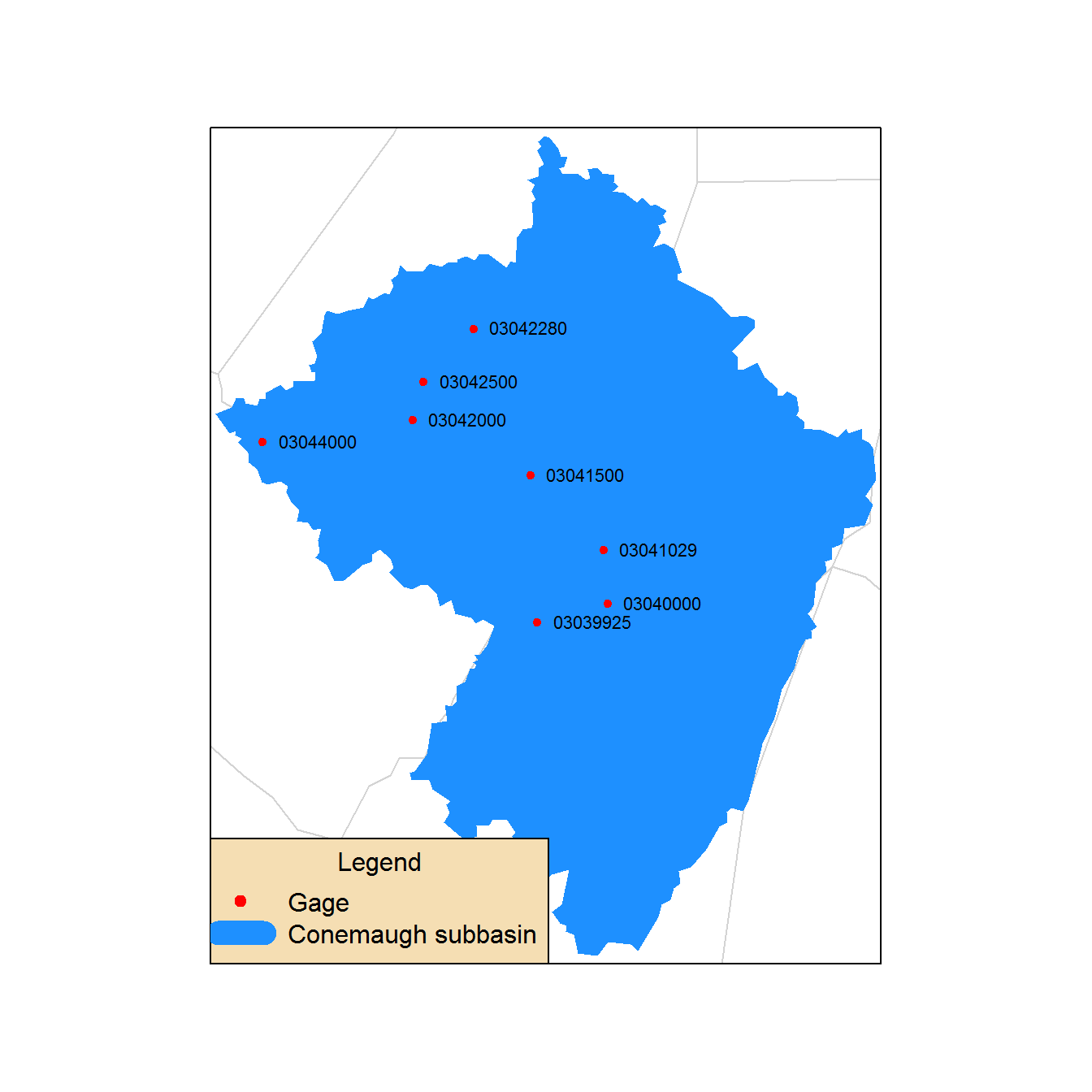
Polygon map zoomed to HUC
Other packages and examples
Like plotting in R, there are endless intricacies to making maps, and we are only really scratching the surface here. Some other packages that you may find useful for certain applications include:
- raster : For working with your own raster data
- sp
: The original workhorse package for handling spatial data.
sfis largely replacing it, but you will see it a lot when Googling things. - geoknife : A USGS package that utilizes the Geo Data Portal for processing gridded data. Covered in the packages curriculum .
- inlmisc : Another USGS package for creating high-level graphics, demonstrated in this post by Jason Fisher .
Also, check out our additional topics in R page for links to some other tutorials.
Categories:
Keywords:
Related Posts
Beyond Basic R - Version Control with Git
August 24, 2018
Depending on how new you are to software development and/or R programming, you may have heard people mention version control, Git, or GitHub. Version control refers to the idea of tracking changes to files through time and various contributors. Git is an example of a version control tool, and GitHub is a popular web interface for Git. That’s it. Easy!
Beyond Basic R - Plotting with ggplot2 and Multiple Plots in One Figure
August 9, 2018
R can create almost any plot imaginable and as with most things in R if you don’t know where to start, try Google. The Introduction to R curriculum summarizes some of the most used plots, but cannot begin to expose people to the breadth of plot options that exist.There are existing resources that are great references for plotting in R:
Beyond Basic R - Data Munging
August 1, 2018
What we couldn’t cover
In the data cleaning portion of our Intro to R class , we cover a variety of common data manipulation tasks. Most of these were achieved using the package
dplyr, including removing or retaining certain columns (select), filtering out rows by column condition (filter), creating new columns (mutate), renaming columns (rename), grouping data by categorical variables (group_by), and summarizing data (summarize).Beyond Basic R - Introduction and Best Practices
July 30, 2018
We queried more than 60 people who have taken the USGS Introduction to R class over the last two years to understand what other skills and techniques are desired, but not covered in the course. Though many people have asked for an intermediate level class, we believe that many of the skills could be best taught through existing online materials. Instead of creating a stand-alone course, we invested our time into compiling the results of the survey, creating short examples, and linking to the necessary resources within a series of posts. This is the first in a series of 5 posts called Beyond basic R.
The Hydro Network-Linked Data Index
November 2, 2020
Introduction
updated 11-2-2020 after updates described here .
updated 9-20-2024 when the NLDI moved from labs.waterdata.usgs.gov to api.water.usgs.gov/nldi/
The Hydro Network-Linked Data Index (NLDI) is a system that can index data to NHDPlus V2 catchments and offers a search service to discover indexed information. Data linked to the NLDI includes active NWIS stream gages , water quality portal sites , and outlets of HUC12 watersheds . The NLDI is a core product of the Internet of Water and is being developed as an open source project. .

